1 Introduction

CVTree (Composition Vector Tree) is an implementation of alignment-free algorithms for generating dissimilarity matrices from large collections of DNA or amino acid sequences, preferably genome data, for phylogenetic studies. This method was proposed by Professor Bailin Hao and colleagues in 2004 (J. Qi, Wang, & Hao, 2004). In the CVTree algorithm, each genome sequence (including protein, RNA, or DNA) is represented by a composition vector, which is calculated by the difference between the observed frequencies of k-strings and the predicted frequencies based on a Markov model. The similarity between two sequences is measured by the cosine of their composition vectors. CVTree has been successfully applied to various domains, including Archaea and Bacteria (Gao, Qi, Sun, & Hao, 2007; J. Qi et al., 2004; Sun, Xu, & Hao, 2010; G. H. Zuo, Hao, & Staley, 2014a; Zuo, Xu, & Hao, 2013, 2015), viruses (Gao & Qi, 2007; Gao, Qi, Wei, Sun, & Hao, 2003), chloroplasts (Yu et al., 2005), 16S rRNA (Lu, 2025), fungi (Choi, Kim, Jeon, & Lee, 2013; O’Connell, Thon, Hacquard, & Amyotte, 2012; Wang, Xu, Gao, & L., 2009), and metagenomes (Liu et al., 2013; Zhang et al., 2016). The methodological aspects of the CV approach have been extensively described in the literature. In particular, the role and selection of the peptide length \(K\) have been discussed in (Li, Xu, & Hao, 2010) and (G. H. Zuo, Li, & Hao, 2014b).

The CVTree algorithms are accessible through two platforms: the CVTree Web Server and the CVTree Standalone Version. The standalone version is published under the MIT license on both GitHub and Gitee (Zuo, 2021). Following the introduction of the classical CVTree method, our research group has successively released three versions of the CVTree web server (Ji Qi, Luo, & Hao, 2004; Xu & Hao, 2009; Zuo & Hao, 2015). In WebCVTree v3 (Zuo & Hao, 2015), we redesigned the data processing strategy and implemented parallelization for the core program. Additionally, an interactive, collapsible, and expandable CVTree Viewer based on HTML5 was incorporated. These enhancements enable biologists to study phylogeny inferred from thousands of genomes and compare results directly with taxonomy at all ranks in an almost automated manner. WebCVTree v4 represents the latest iteration of the CVTree Web Server. This version incorporates all prokaryotic genomes from NCBI RefSeq, features an improved data processing strategy, introduces a novel algorithm for comparing phylogenetic trees with taxonomy, and implements more efficient core programs. In addition to the interactive HTML5-based Tree Viewer from WebCVTree v3, a new tree drawing page has been added to generate publication-quality phylogenetic tree figures. The WebCVTree4 pipeline is hosted on Aliyun and accessible at http://cvtree.online/v4/. The WebCVTree4 web server can be accessed without login requirements on most modern browsers, including Firefox, Microsoft Edge, and Google Chrome. However, due to HTML5 implementation, some older browsers may not be fully supported.

1.1 New Features in WebCVTree v4

1. Integrated Taxonomy System: Implementation of a comprehensive taxonomy system based on the NCBI taxonomy database.
2. Comprehensive Prokaryotic Genomes: Inclusion of all RefSeq prokaryotic genomes for comprehensive analysis.
3. Phylogenetic Tree Editor: Built-in functionality for editing and customizing phylogenetic trees.
4. Detailed Lineage Editor: Advanced editor for modifying the taxonomic lineage of individual genomes.
5. Novel Comparison Algorithm: Implementation of a new algorithm for comparing phylogenetic trees with taxonomic classifications.
6. Enhanced Taxonomy Display: Updated visualization system for improved taxonomic data presentation.
7. New Web Infrastructure: Deployment on a new server infrastructure hosted on Aliyun at http://cvtree.online/v4/.
8. Optimized Server Performance: Implementation of more efficient server-side programs for enhanced computational speed.

1.2 Citation Guidelines

When using WebCVTree in your research, please cite the following relevant publications:

1. Zuo, G. (2025). WebCVTree4: A Novel Phylogenetic and Taxonomic Study Platform for Prokaryotes Using Composition Vectors and Whole Genomes. In Submission.
2. Zuo, G. (2025). CLTree: Annotating, Rooting, and Evaluating Phylogenetic Trees Based on Genome Lineages. In Submission.
3. Zuo, G. (2021). CVTree: A Parallel Alignment-free Phylogeny and Taxonomy Tool Based on Composition Vectors of Genomes. Genomics Proteomics & Bioinformatics, 19, 662-667.
4. Qi, J., Wang, B., & Hao, B. (2004). Whole proteome prokaryote phylogeny without sequence alignment: a K-string composition approach. Journal of Molecular Evolution, 58, 1-11.

2 Web Interface

The workflow of WebCVTree v4 is illustrated in Figure 1.

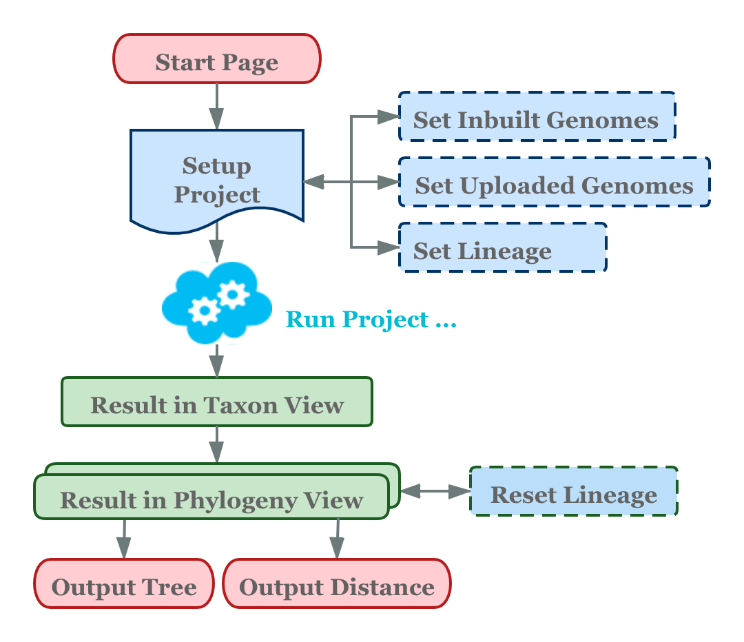
The operational workflow of WebCVTree consists of three main stages: project initiation from the Home Page, parameter configuration and job submission. The parameter configuration encompasses four components: basic parameters (configured in the Project Page), selection of built-in gene sequences (configured in the Inbuilt Page), uploading of external gene sequences (configured in the Upload Page), and setting of genome classification information (configured in the Lineage Page). Once all parameters are configured, the job can be submitted to the server for processing. Upon completion, results are presented from two perspectives: taxonomic classification (TaxonView Page) and phylogenetic tree visualization (TreeView Page). Users can generate publication-ready, high-quality figures directly from the system for use in academic publications via the Output Tree page. For users interested in numerical values representing distances between specific species, this information is available on the Output Distance page. Furthermore, if the classification or phylogenetic tree results are unsatisfactory, users have the flexibility to modify the classification information and re-run the comparison between lineage and phylogenetic tree to iteratively refine their results.

2.1 Getting Started

The Start Page of WebCVTree4 is illustrated in Figure 2. To reload an existing project, enter its Project Number in the designated textbox and click the Load/Create Project button. To initiate a new project, leave the textbox empty and click Load/Create Project. Each user job is assigned a unique Project Number, and a dedicated workspace is allocated to the project. All project configurations, user-uploaded data, and computational results are stored in this workspace. Projects and their associated workspaces are retained for 7 days following the most recent run.

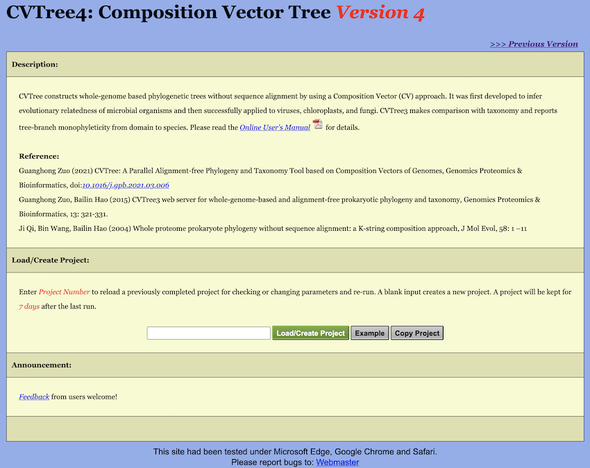
Adjacent to the Load/Create Project button is a button labeled Example. Clicking this button displays a preset example project that was utilized in the publication describing WebCVTree4. First-time users are strongly encouraged to explore this example to gain a comprehensive understanding of WebCVTree4’s functionality and workflow.

Next to the Example button is a button labeled Copy Project. Clicking this button duplicates a preset project into a new project with a unique Project Number. WebCVTree4 supports an incremental computational workflow by enabling users to replicate existing projects, modify parameters, and execute new runs that utilize previous results. This approach prevents unnecessary repetitive calculations and improves computational efficiency. Furthermore, by preserving all uploaded data within the project structure, the Copy Project functionality eliminates redundant data upload procedures. Note that a valid existing Project Number must be entered in the textbox before clicking the Copy Project button.

2.2 Setting Up A Project

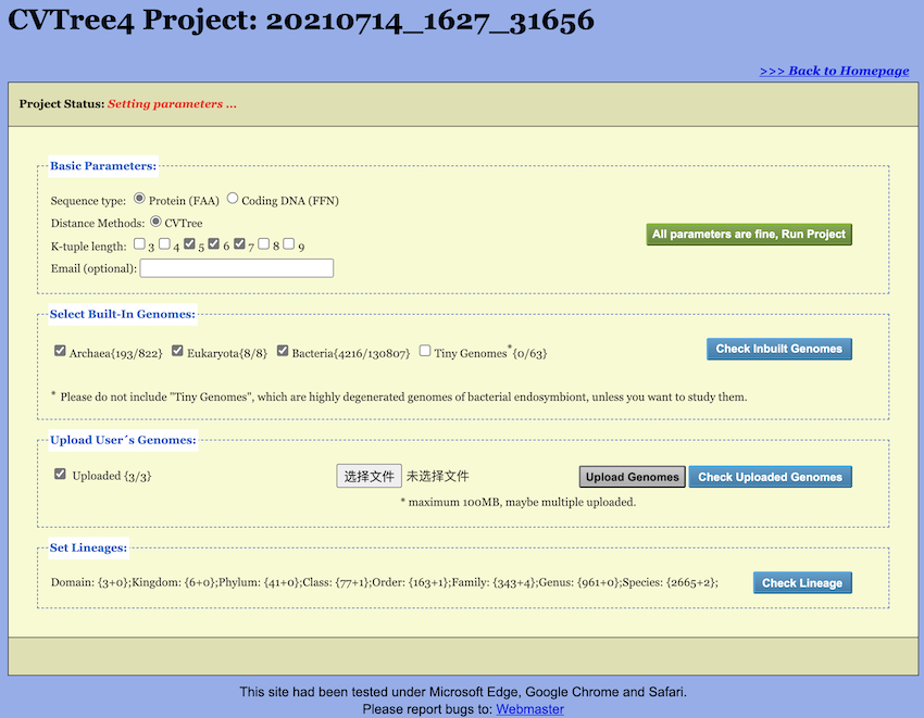
Upon creating, loading, or copying a project, the Setup Page opens in the “Setting parameters” status (see Figure 3). The unique Project Number is displayed at the top of the page; users should retain this number for subsequent project access. The Setup Page begins with a Project Status bar indicating the current status of the project (see Figure 4). The main section of the Setup Page comprises three primary sections: Basic Parameters, Set Genomes, and Set Lineage.

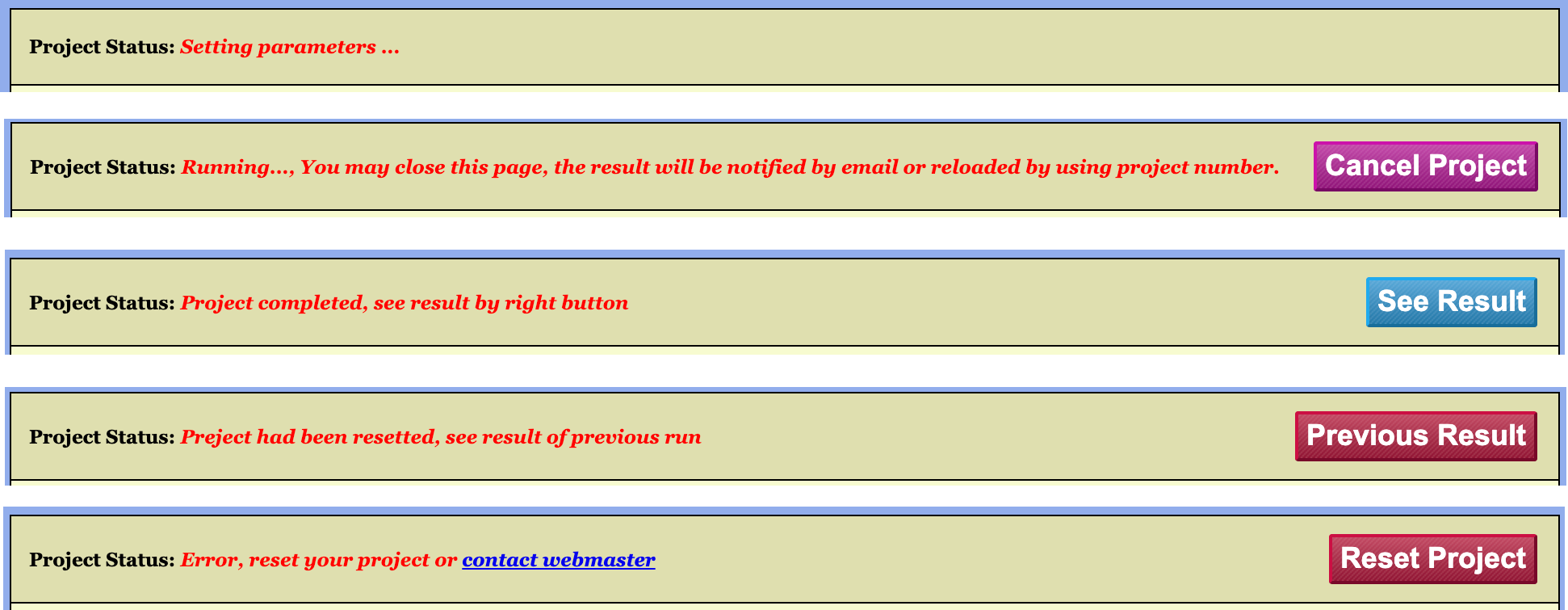
2.2.1 The Project Status Bar

As illustrated in Figure 4, a project may exist in one of the following five states:

1. Initial State: The project is awaiting parameter configuration and job submission.
2. Running State: The project has been configured and submitted to the server, which is currently processing the job. In this state, the configuration interface is locked. A Cancel Project button appears on the right side of the Project Status Bar; clicking this button terminates the running task and unlocks the interface.
3. Completed State: The server has finished processing the job and successfully returned the results. In this state, a See Result button appears on the right side of the Project Status Bar, providing access to the results page.

In addition to the three normal workflow states described above, there are two exceptional states:

4. Project Reset: A new configuration has been applied to an already completed project and saved to the server, but not yet resubmitted. An example would be generating a new project via the Copy Project function and subsequently modifying its parameters.
5. Runtime Error: An error occurred during server processing due to specific issues. The configuration interface remains locked, and a Reset Project button appears on the right side of the Project Status Bar to exit the locked configuration state.

2.2.2 Basic Parameters

Users configure Basic Parameters in the “Basic Parameters” section of the Setup Page.

1. Sequence Type: Although protein sequences are preferred, DNA sequences may also be used.
2. Distance Method: Currently, WebCVTree4 provides only the classic CVTree method, also referred to as the “Hao method” in the new CVTree software. Users wishing to employ other CVTree methods should utilize the local version of the software, whose source code is available for download on both GitHub and Gitee. For detailed algorithmic information, please refer to the reference document (Zuo, 2021).
3. K-tuple Length: WebCVTree4 can generate trees for all selected K-tuple lengths in a single run. The default K-values range from 5 to 7 for proteins and from 6 to 18 with increments of 3 for coding DNAs, though any single K-value may be selected. When using protein sequences, the optimal K range is 4-5 for viruses, 5-6 for prokaryotes, and 6-7 for fungi (Li et al., 2010). K-values of 8 and 9 are available but generally unnecessary.
4. Email: Users may optionally provide an email address to receive notification when the project is completed. Alternatively, results can be reloaded at a later time using the Project Number as described above.

2.2.3 Choosing Inbuilt Genomes

The WebCVTree4 web server incorporates a comprehensive built-in database of genomes, which are categorized into several groups as indicated by the selectable buttons: Archaea (1,154 genomes), Bacteria (223,734 genomes), Tiny Genomes (81 genomes), and Eukarya (8 genomes). The numerals in parentheses represent the number of genomes within each group. For additional information regarding these genome categories, please refer to Section 3.1. Users can select inbuilt genomes through two methods:

1. By clicking the checkbox preceding each group, users can select or deselect an entire group. The outgroup will be automatically selected by the web server.
2. If a user wants to select genomes one by one and set an outgroup by oneself, please get into the Select Inbuilt Genomes Page by clicking on the Check Inbuilt Genome button.

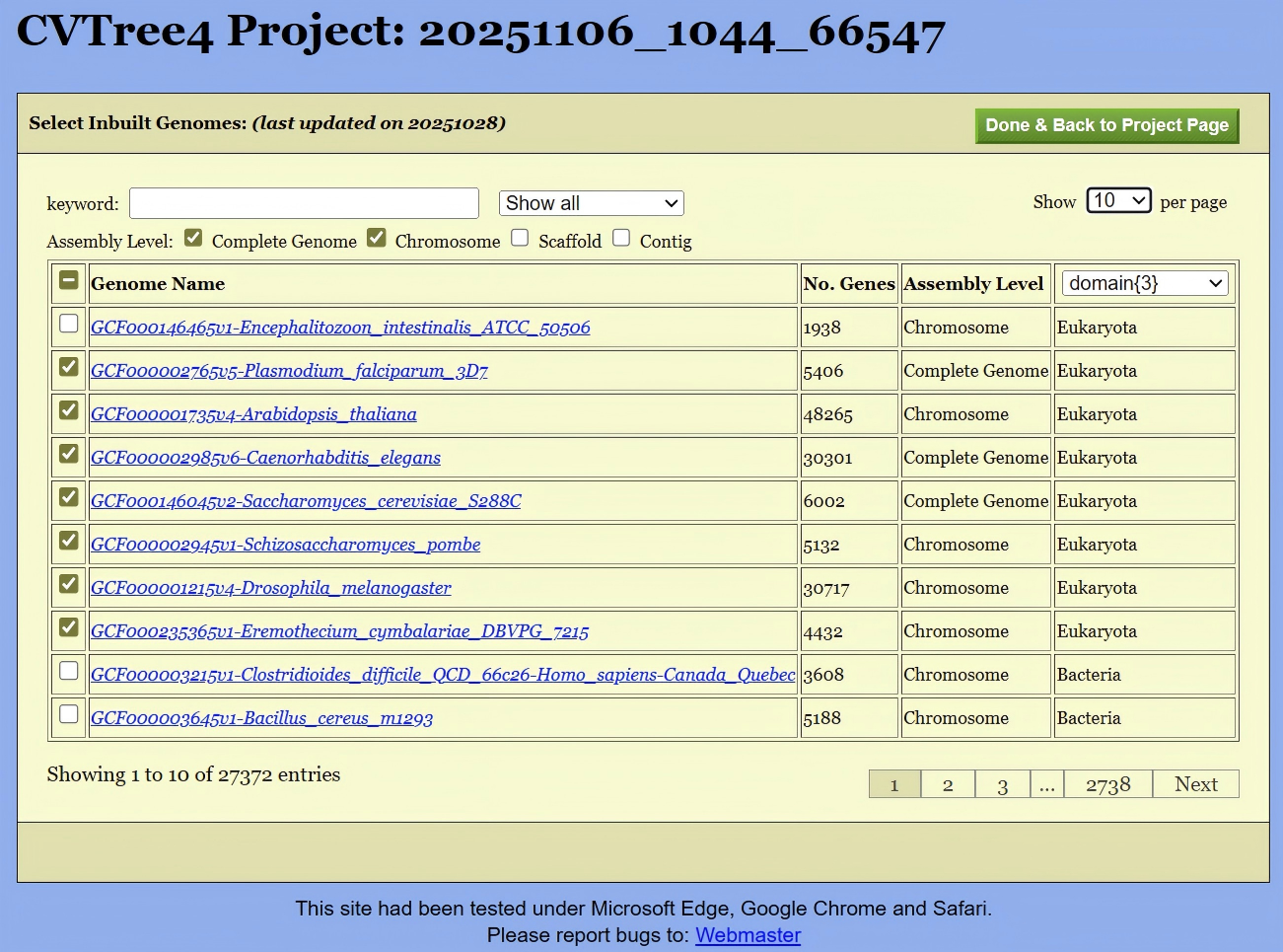
This Inbuilt Genomes page (shown in Figure 5) consists of a long list of all builtin genomes. The first column is the checkbox for select the inbuilt genomes into the project. Entries in this table is sortable by clicking on the head of the table. For example, by clicking on “Genome Name”, all the genomes would appear in alphabetic order of their names; by clicking on “No. Genes”, the genomes will be ordered by the total number of genes.

The subsequent row pertains to the assembly level. As per NCBI information, there are four defined assembly levels (“Complete Genome”, “Chromosome”, “Scaffold”, “Contig”). A filter located above the table enables users to display only genomes of superior assembly quality, thereby avoiding the potential for lower-quality genomic sequences to introduce errors into the overall computational results.

The last column of the table possesses a pull-down list of taxonomic ranks with number of taxa in each rank: from Domian{3} to Species{34478} for the time of writing these lines. A user can pick up an item from the list to facilitate the selection of genomes.

After completing the selection one returns to the Project page (Figure 3) by clicking on Done & Back to Project page.

2.2.4 Upload Genomes

Upon clicking the Upload User's Genomes button, you can select the genome files for upload. Two important points to note here: first, you can select multiple genome sequences at once; second, the file extensions of the uploaded genomes must match the genome type selected in the Basic Parameters section, i.e. .faa for protein sequences or .ffn for the DNA sequences.

After the genomes are successfully uploaded, the “Uploaded” checkbox will display the count of uploaded genomes. Similar to the representation for built-in genomes, the number before the ‘/’ indicates the count of selected genomes in the follow calculation, and the number after the ‘/’ shows the total number of uploaded genomes. All user genomes, checked or unchecked, together with the configured project will be kept for 7 days after the last run.

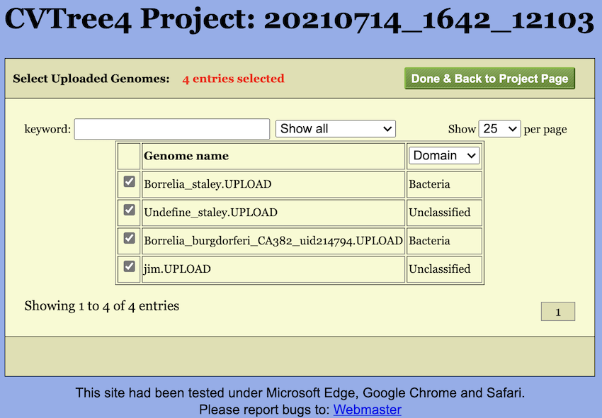
Furthermore, once genomes are uploaded, a small blue tag will appear next to the checkbox. Clicking this tag opens a selection page (see Figure Figure 6) where you can choose which genomes to include in the calculation. By default, all uploaded genomes are selected.

Additionally, it should be noted that after upload, the genome names will be appended with an ‘UPLOAD’ suffix to distinguish them from the built-in genomes. Similarly, you can also choose to calculate only the uploaded genomes by unchecking the “Uploaded” checkbox.

2.2.5 Set Lineages of Genomes

The handling of Lineage information represents one of the most significant upgrades in WebCVTree4 compared to its previous version. In WebCVTree4, the lineage information for selected built-in genomes is pre-processed. For user-uploaded genomes, the system attempts to infer a possible lineage based on the file name by referencing NCBI taxonomy data. If the classification is unclear, the genome is labeled as “Unclassified”.

In summary, if no additional action is taken by the user, the system will automatically process all lineage information once the job is submitted. However, if users wish to preview the classification information in advance, they can click the Update Lineage button. The server will then update the lineage information for all selected genomes and display the counts for each taxonomic level in the Set Lineages block. Here, the number before the “+” indicates the count of genomes with a known classification at that level, while the number after the “+” shows how many genomes are currently “Unclassified” for that level.

To examine the detailed lineage information, users can click the Check Lineage button, which will bring up a page from the server as shown in Figure 7.

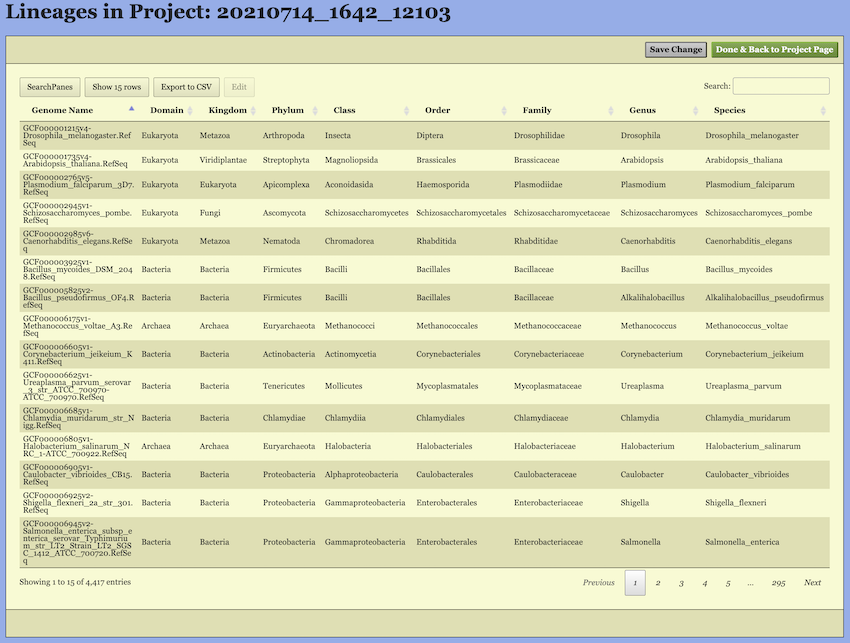
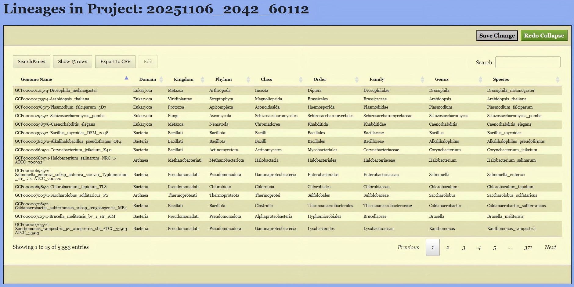
Upon entering the “Lineage Page”, the taxonomic information for all selected genomes—including both built-in and user-uploaded genomes—is displayed in a table.

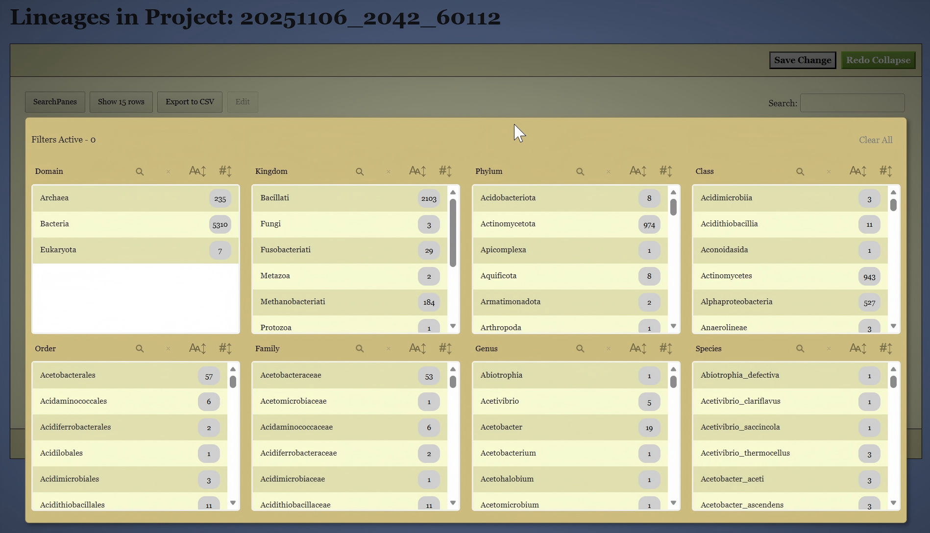
On this page, you can filter the genomes based on their existing classifications. To do this, click the “SearchPanes” button to reveal all available taxonomic categories, as shown in Figure 8. The interface will then allow you to select specific taxa at each classification level to narrow down the genomes of interest. You can also use the search box on the right side to search the genomes by keywords.

These classification details can be manually modified in two ways:

1. Offline Editing via CSV Export: Click the Export to CSV button to download the entire table as a CSV file. You can edit the file locally using spreadsheet software and then upload the modified file back to the page via drag-and-drop.

2. Online Editing: Select one or more genomes in the table to activate the Edit button. Clicking it will open a pop-up dialog (shown in Figure 9). In this dialog, the lineage information for all selected genomes is merged. If all selected genomes share the same name at a specific taxonomic level, that name is displayed. If there are multiple different names, “Multi-valued” is shown instead. You can edit these names, and your changes will apply to the corresponding taxonomic level.

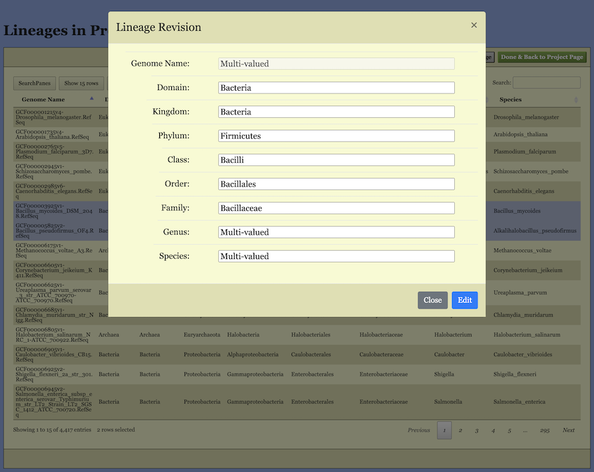
Important Note Regarding “Multi-valued”: If you leave a “Multi-valued” entry unchanged, the original distinct names for that level will be preserved for their respective genomes. However, if you enter a new name, it will overwrite and unify the taxonomic level for allselected genomes.

2.3 Run Project

When all paramenters are set the project is submitted for processing by clicking the button All parameters are fine, Run Project at the right side of basic parameters block (see Figure 3). After submission the “Setting parameters” status will be locked and the project status changes to that shown in the middle of Figure 4, namely, “Running \(\cdots\)”. The project will be done in a few minutes if only the inbuilt genomes are used. If many new genomes are uploaded, the waiting time might be much longer, depending on the size and number of genomes. One can safely close the page and the completion of job be notified later by email if an email has been entered when setting parameters. And users can also revisit the web server and reload the project by entering the Project Number. And if necessary one can cancel the project and reset parameters by clicking the button Cancel Project and reset the project.

When the project is completed, the Project Status bar changes to that shown in the third block of Figure 4. By clicking on the See Result button one is led to the Result Page. It shown be noted that, regarding the validation of the generated phylogenetic tree, we believe that the approach should not be limited to simple sampling tests, as the results obtained from such methods only demonstrate the self-consistency of the data. Instead, we advocate for the use of validation methods that are independent of the current dataset. Through years of research, we have found that comparing taxonomic information with phylogenetic relationships serves as an exceptionally effective validation technique. To this end, we have developed a novel algorithm that annotates the phylogenetic tree with taxonomic information, enabling a comprehensive comparison between the taxonomic system and the inferred phylogenetic relationships. For a detailed explanation of the algorithm and its underlying concepts, please refer to Section 4.2. The following section will focus on how these results are presented on the web interface. Overall, the presentation is divided into two perspectives: one based on the taxonomic view and the other based on the phylogenetic tree view.

2.4 Taxon View Page

The Result Page almost entirely consists of a long table summarizing taxa convergence except for two buttons in the upper-right corner: See Tree and Download Result. Here See Tree is the portal to the interactive tree display to be described in Section 2.5, Download Result is where the user can download the results to the local computer for further analysis and archiving. It may be used any time while on-line or after reloading a project.

The interface then presents three tabs: By Lineage, By Level, and Unclassified. In our process of comparing the phylogenetic tree with the taxonomic system, we treat genomes with unknown taxonomic units—specifically those labeled as Unclassified—separately from genomes that have complete taxonomic information. Therefore, the first two tabs (By Lineage and By Level) present the comparison between the phylogenetic tree and the taxonomic system for genomes with complete classification, but from two different perspectives. The Unclassified tab displays genomes with incomplete taxonomic information. If no genomes in the project lack classification data, this tab will not appear.

2.4.1 Summary of Taxa by Lineage

On the By Lineage Tab of this page, the taxonomic levels are displayed in a hierarchical order (see Figure 10). For clarity, when the page is first opened, all taxonomic units are collapsed to the highest level. Clicking the triangle (\(\blacktriangleright\)) next to a unit expands it to reveal the subordinate taxonomic levels, and the triangle icon rotates downward (\(\blacktriangledown\)). You can also search for specific taxonomic units using the search box at the top, or select a specific taxonomic level from the dropdown menu to collapse the hierarchy to that chosen level.

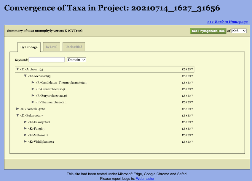
Convergence of taxa at various K-values provides an additional angle to look at the phylogeny. That is why WebCVTree4 calculates trees at several Ks in one run and produces a summary report. In the taxonomic view, the comparison results under different K-values are consolidated and displayed together. As illustrated in the figure, each taxonomic unit is represented in the following format:

<P>Bacillota:1105                --K6K7

A taxon name is followed by the number of genomes belonging to the taxon. Before the taxon name is the abbreviation of the taxon rank. Here, abbreviations are used for the ranks: \(<\)D\(>\) Domain, \(<\)K\(>\) Kingdom, \(<\)P\(>\) Phylum, \(<\)C\(>\) Class, \(<\)O\(>\) Order, \(<\)F\(>\) Family, \(<\)G\(>\) Genus, and \(<\)S\(>\) Species. The same set of abbreviations with an additional \(<\)T\(>\) for sTrains are used in the CVTree Viewer. And then is the taxon name. The monophyly status of the taxon is given at the right. For example, there are 1105 genomes for the archaeal phylum Bacillota and it is monophyletic at all K’s except for \(K=6\) and \(K=7\), but not in \(K=5\).

2.4.2 Summary of Taxa by Taxon Level

As shown in the figure, the “By Level” tab displays the comparison results organized by taxonomic rank and provides corresponding statistics (See Figure 11). On this page, users can utilize the dropdown menu to filter and display items of a specific category. The number following each taxonomic rank is formatted as X / Y. Here, the number after the slash (/) indicates the total number of itemsbelonging to that rank, while the number before the slash represents the count of items matching the currently selected category. The detailed Monophyly status of individual items is displayed in the same manner as in the By Lineage Tab. Furthermore, you can click on any taxonomic rank to view its detailed information.

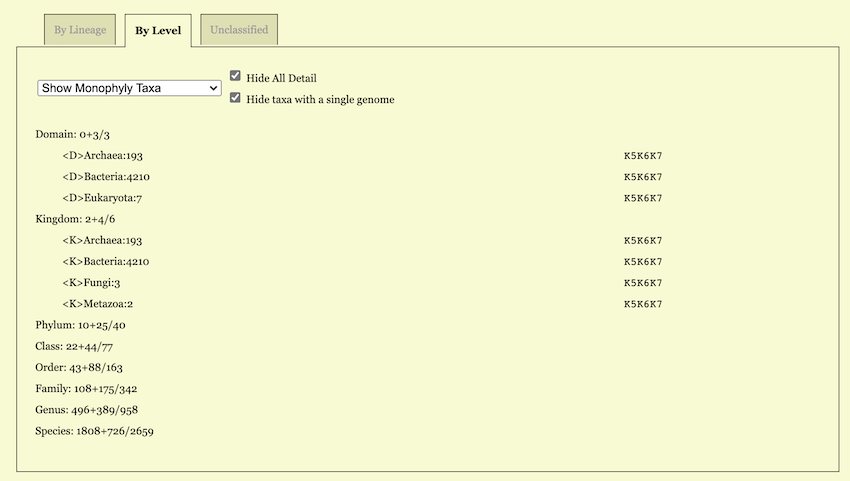
For example, when “Show Monophyly Taxa” is chosen, each taxonomic rank as a subtitle carries a statistic. For example, a line

Phylum: 5+35/41

tells that the total number of classes is 41 in the input dataset (after taking into account taxonomic revision, if any); among these 41 classes 5 are represented by only one genome hence are trivially monophyletic; the other 35 are represented by two or more genomes and are monophyletic at least for one K.

In the “Show Non-Monophyly Taxa” option, the corresponding line reads

Phylum: 1/41

indicating that there are \(41 - 5 - 35 = 1\) classes, which are not monophyletic for whatsoever K. In a sense, these non-monophyletic taxa are worth further studying as they may hint on possible taxonomic revisions.

2.4.3 Summary of Unclassified Genomes

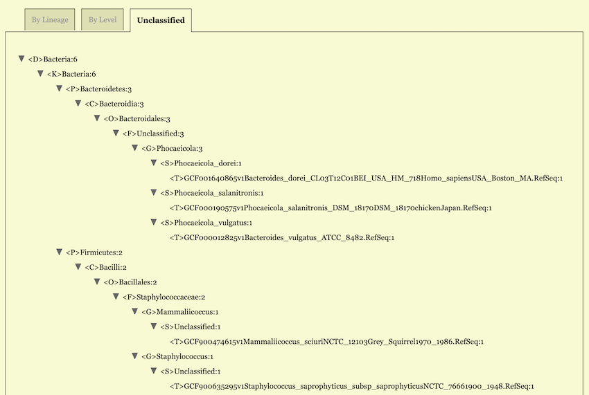
Items that lack classification information are grouped and displayed in a separate tab labeled Unclassified, as illustrated below Figure 12. This helps to look for taxa with incomplete lineage information.

2.5 Tree View Page

It is extremely difficult, if not impossible, to comprehend a tree made of thousands of leaves. To this end an interactive, collapsible and expandable, display has been developed since WebCVTree3. As skillful manipulation of the display is the key point to make the most of WebCVTree4. Therefore, we explain the interactive display in more details.

By clicking the button See Tree in the upper-right corner of the Result Page (see Figure 10), a TreeViewer page with default \(K=6\) opens up.

A typical tree, plotted by using HTML5, is shown in Figure 13.

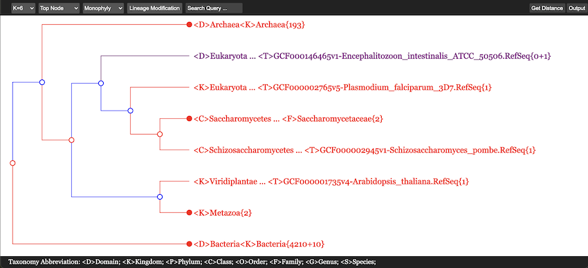
First of all, in Figure 13 all 235 Archaea, 5310 Bacteria and 8 Eukarya genomes are accomodated within a single screen. The {n + m} convention in number of genomes will be explained later. This picture was obtained after searching for the class name “Lactobacillales” and only its neighborhood has been expanded somehow, while all other branches were maximally collapsed except for one line exposed in purple. In total, four colors are used in this figure. Their meaning will be explained in the next subsection.

2.5.1 Circles in Tree

If a node is denoted by a blank circle (\(\circ\)), it is collapsible. One may click on the circle to have all the lower branchings shrinked; the collapsed branch is labeled by the highest-rank common taxon name. At the lowest level, a rightmost node may be marked by a solid circle (\(\bullet\)) preceding a taxon name; it tells that there are more than one genomes in that branch and it may be expanded by clicking on the solid circle. In contrast, a short line (—) in place of a would-be circle means that there is only one genome and it cannot be further expanded.

2.5.2 Color of Items

Taxon names may appear in one of four colors: red, blue, green and purple.

1. A red name indicates that the branch is monophyletic and collapsed. This includes the trivial case when a taxon is represented by a single genome. For example: <D>Archaea{235}.
2. A collapsed but not convergent branch such as <K>Pseudomonadati{503/3107} is shown in blue.
3. A taxon name in green matches the word a user types in place “Search Query”, i.e., <O>Lactobacillales in this picture.
4. Purple color is used to show a taxon with incomplete lineage information, with “Unclassified” items. In Figure 13 there is only one line in purple: <D>Eukaryota ... <T>GCF000146465v1-Encephalitozoon_intestinalis_ATCC_50506{0+1}.

2.5.3 The Taxonname {n + m } Convention

A taxon name such as <D>Eukaryota{7+1} indicates that 1 of the 8 bacterial genomes did not come with complete lineage information. Only taxa with complete lineage information are counted in the convergence report as an augend {n, while genomes without complete lineage information are indicated in the tree display as an addend +m}. This convention is useful for studying taxonomic assignment of newly sequenced genomes without proper lineage information. However, please note that lineage information for a given taxon may be complete but incorrect, thus requiring further modification.

2.5.4 Select Another Tree

A toolbar at the top of the page provides buttons for performing specific operations. The first button allows you to open phylogenetic trees generated under different K-values within this same page.

2.5.5 Select Root Node

One can pick up a branch and let it fills up the whole display window. For example, to single out the domain <D>$Archaea{235} one holds the shift key and clicks on the solid circle in front of the species name. The leaf \(\bullet<\)S\(>\)Archaea{235} will move to the leftmost position in the display and further clicking on the solid circle expands it to the whole window.

The aforementioned operation of picking up a branch may be performed in another way, namely, by using the “Select Node” option in the headline of the CVTree Viewer. By selecting a taxon name in the pull-down list, e.g., <P>Methanobacteriota:178, the phylum Methanobacteriota represented by 178 genomes for the time being is displayed in the whole window.

2.5.6 Display Style

In addition to expanding or collapsing branches on the phylogenetic tree by clicking the circles on the nodes, you can also perform bulk operations using the third button. For example, you can collapse the entire tree to a specific taxonomic rank, or display all items labeled as “Unclassified” or “Upload”.

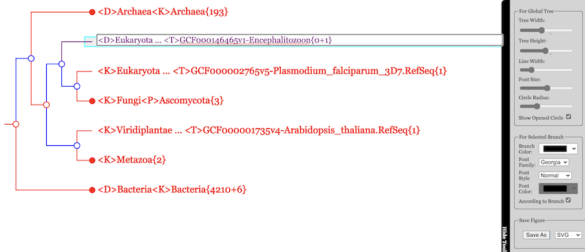
2.5.7 Lineage Revision

The option “Lineage Modificaion” in the CVTree Viewer provides this function. By clicking on this option an empty “Lineage Modification” window opens up: it looks like Figure 14. This page is essentially the same as the “Check Lineage” page in the project settings, with the exception of the Redo Collaps button in the upper-right corner. Its operation is also consistent with the description in Section 2.2.5. When a Lineage Modification file is ready, one clicks on the Redo Collapse button in top-right. The system shows “Recollapsing is running. Please wait.” It takes a minute or two. Then it says “Recollapse successfully”. Both the taxa convergence table and the CVTree Viewer have been renewed. We emphasize that actual taxonomic revisions must comply with the International Code of Nomenclature of Bacteria (Lapage, Sneath, & Lessal, 1992) and follow the established practice in the microbiological community. The Lineage Modificarion function provided by WebCVTree4 is solely for trial purpose.

2.5.8 Search Query

The quickest way to get to the point of interest in a tree is typing a taxon name in place of the “Search Query”. For example, one may type “Escherichia” and select an item from the pull-down list, e.g., Escherichia_coli.

2.6 Output and Edit Tree

When a tree view has been adjusted by appropriately collapsing and expanding, a print quality figure can be obtained by clicking on the output button in the upper-right corner of the CVTree Viewer page (Figure 13). It opens an output preview page (Figure 15). The main options for tree is:

1. On the right side of the page, there is a collapsible control panel. Using this panel, users can modify various aspects of the phylogenetic tree, such as tree style, branch lengths and spacing, text size and font, the colors of branches and labels, the display of collapsed branches, and the circles on nodes, and so on.
2. Click on the branch to select the brach, and the change the style, color and font style by the right pannel.
3. Double click the name of the terminal node, you can change the name of the branch.
4. Holding down the Shiftkey and clicking on a specific node, you can swap the two branches (clades) that descend from it.

A useful tip: When selecting branches, it can be difficult to click on the thin lines. While adjusting the figure, keep the open circles on the branches enabled for easier selection. You can remove them in the final step before exporting by the right pannel.

With the adjustments described above, it is generally possible to generate a phylogenetic tree figure suitable for publication. And then, one may select a format to save a figure. The default format is SVG (Scalable Vector Graphics), as the underlying plot is done in SVG. One may save the figure into PDF, eps, and png formats as well.

2.7 Obtain Distance between Genomes

To optimize storage efficiency and accelerate computation, the distance files generated by the CVTree software are not saved in a standard format and require specialized commands for parsing. Consequently, WebCVTree does not provide an option to download these distance files.

For users who are interested in the specific numerical distances and wish to conduct repeated comparative analyses, we recommend running CVTree locally. The software can be easily downloaded from GitHub or Gitee. Additionally, a containerized version compatible with Singularity is available, which eliminates the need for complex compilation steps.

However, as a temporary solution within WebCVTree4, we do provide a method to access the distance matrix generated during the CVTree calculation process.

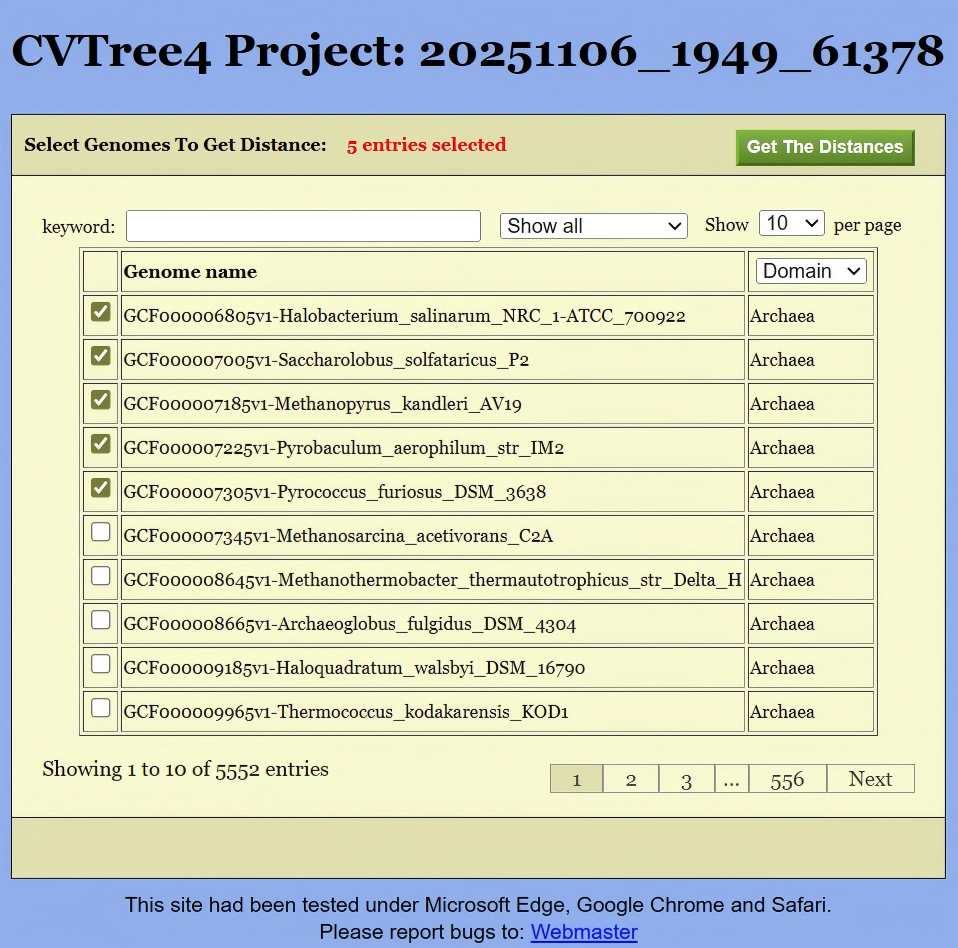
To obtain the distance matrix, the first step is to select the target genomes. This can be done in either of the following two ways:

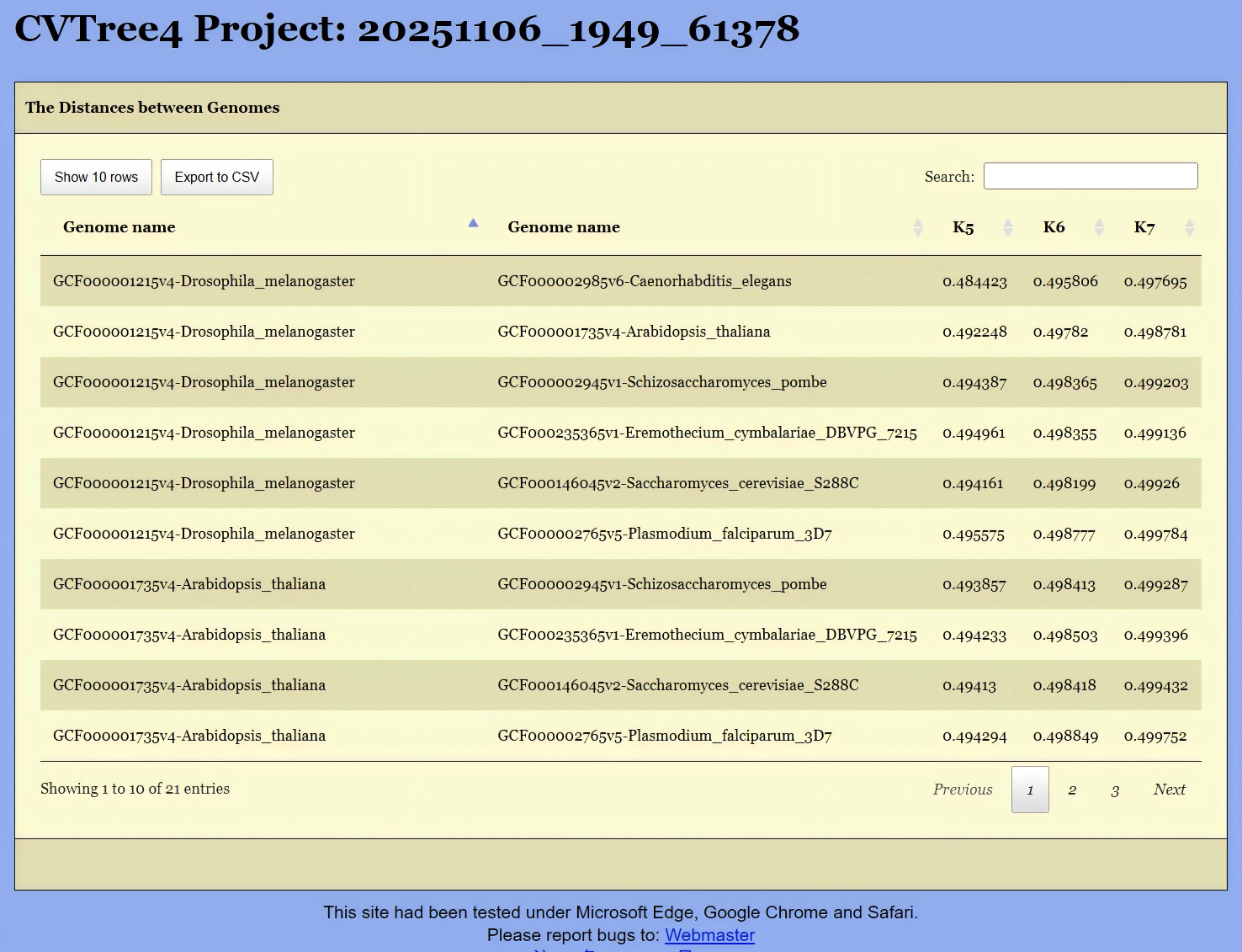
1. Click the Get Distance button located in the upper-left corner of Figure 13. This will open the interface shown in Figure 16, where you can select the relevant genomes. Then, clicking Get the Distance will generate a distance list, as displayed in Figure 17. This list can be exported as a CSV file for further analysis.

2. Alternatively, if you are interested in the distances between species under a specific branch, you can hold down the Altkey and click on the corresponding node in the phylogenetic tree shown in Figure 13. This will also generate the same distance list, like Figure 17.

3 Inbuilt Data

3.1 Inbuilt Genomes

3.1.1 Prokaryotic Genomes

The WebCVTree4 webserver inbuilt all prokaryotic genomes of the NCBI RefSeq database.

1. Archaea of Refseq NCBI: ftp://ftp.ncbi.nih.gov/genomes/refseq/archaea
2. Bacteria of NCBI RefSeq: ftp://ftp.ncbi.nih.gov/genomes/refseq/bacteria

3.1.2 Eukaryote Genomes

Eight eukaryotic genomes, 4 fungal and 4 non-fungal, are provided for serving as outgroup in tree construction. The non-fungal genomes are Caenorhabditis elegans, Arabidopsis thaliana, Plasmodium falciparum and Drosophila melanogaster.

3.1.3 Tiny Genomes

There are a few highly degenerated genomes of bacterial endosymbiont bacteria in the in-built database. Their proteomes are very small (\(< 10000\) amino acids), hence the adjective “Tiny”. Due to lacking of many genes the position of these species in the phylogeny often turns out to be questionable, e.g., they tend to the root and occasionally violate the trifurcation of the three main domains of life. This is why we suggest not to include the “Tiny Genomes" in a study of mostly”free-living” organisms.

On the other hand, if one is interested in these highly degenerated genomes, then it should be reminded that the cut-off at \(10^4\) amino acids is artificial and many slightly larger genomes, i.e., those from some insect symbionts in the family Enterobacteriaceae must be taken into account as well.

3.2 Taxonomic References

For prokaryotes direct comparison with taxonomy has become feasible only quite recently. On one hand, the completion of the second edition of The Bergey’s Manual of Systematic Bacteriology (Bergey’s Manual Trust, 2001-2012), which has been considered by many microbiologists as the best approximation to an official classification (Konstntinidis & Tiedje, 2005), provides a state-of-the-art framework for taxonomy together with current literature such as as IJSEM International Journal of Systematic and Evolutionary Microbiology. On the other hand, the development of the CVTree approach has provided prokaryotic phylogeny a convenient and comprehensible platform (Hao, 2011; Li et al., 2010).

Speaking about taxonomy one must admit that there is no generally accepted standard for prokaryotic taxonomy. The temptation to become a standard makes the Bergey’s systematics a more conservative source. For example, there were deadlines and other restrictions for inclusion in The Manual. Many newly sequenced genomes do not have neither a standing in bacterial nomenclature nor a validly published name. These organisms are not reflected in Bergey’s Manual or in current literature. In contrast, the NCBI taxonomy, though disclaimed to be a taxonomic reference, is, in fact, more dynamic and up-to-date. At least, for any sequence deposited into GenBank there is a piece of lineage information in NCBI taxonomy, no matter how incomplete it might be. Therefore, WebCVTree4 takes initial lineage information from NCBI.

4 Algorithm

Behind WebCVTree are two core algorithms: CVTree and CLTree.

• CVTree (Compsition Vector Tree): starts with genomic sequences and constructs a phylogenetic tree using a model based on K-mer frequencies.

• CLTree (Collapse Lineage Tree): on the other hand, is an algorithm that compares the phylogenetic tree with a taxonomic system. It annotates the phylogenetic tree with taxonomic information. Furthermore, based on this taxonomic information, CLTree determines a suitable root for the unrooted tree.

4.1 CVTree: Composition Vector Tree

As the CVTree method has been extensively documented in the literature (Hao, 2011; Li et al., 2010; J. Qi et al., 2004), we present only a brief overview here.

4.1.1 Frequency or Probability of Appearance of K-Strings

The alignment-free approach of genome comparison is realized by extending
single nucleotide or single amino acid counting to that of longer K-strings. Among early work along this line we mention the use of dinulceotide relative abundance as a genomic signature (Karlin & Burge, 1995). Given a DNA or amino acid sequence of length \(L\), we count the number of appearance of (overlapping) strings of a fixed length \(K\) in the sequence. The counting may be performed for a complete genome or for a collection of translated amino acid sequences. There are in total \(N\) possible types of such strings: \(N=4^K\) for DNA and \(N=20^K\) for amino acid sequences.

For concreteness consider the case of one protein sequence of length \(L\). Denote the frequency of appearance of the \(K\)-String \(a_1a_2 \cdots a_K\) by
\(f(a_1a_2 \cdots a_K)\), where each \(a_i\) is one of the 20 amino acid single-letter symbols. This frequency divided by the total number \((L-K+1)\) of \(K\)-Strings in the given protein sequence may be taken as the probability \(p(a_1a_2 \cdots a_K)\) of appearance of the string \(a_1a_2 \cdots a_K\) in the protein: \[p(a_1a_2 \cdots a_K)=\frac{f(a_1a_2 \cdots a_K)}{(L-K+1)}\] The collection of such frequencies or probabilities reflects both the result of random mutations and selective evolution in terms of \(K\)-strings as building blocks.

4.1.2 Subtraction of Random Background

Mutations happen in a more or less random manner at the molecular level, while selections shape the direction of evolution. Neutral mutations lead to some randomness in the \(K\)-string composition. In order to highlight the selective diversification of sequence composition one must subtract a random background from the simple counting results. This is done as follows.

Suppose we have done direct counting for all strings of length \((K-1)\) and \((K-2)\). The probability of appearance of \(K\)-strings is predicted by using a Markov model: \[p^0(a_1a_2 \cdots a_K) = \frac{p(a_1a_2 \cdots a_{K-1})p(a_2a_3\cdots a_K)}{p(a_2a_3 \cdots a_{K-1})}\] The superscript 0 on \(p^0\) indicates the fact that it is a predicted quantity. We note that the denominator comes from the frequency of \((K-2)\)-strings. This kind of Markov model prediction has been used in biological sequence analysis since long (Brendel, Beckmann, & Trifonov, 1986). It can be justified by virtue of a maximal entropy principle with appropriate constraints (Hu & Wang, 2001).

4.1.3 Composition Vectors and Dissimilarity Matrix

It is the difference between the actual counting result \(p\) and the predicted value \(p^0\) that really reflects the shaping role of selective evolution. Therefore, we collect \[a_i(a_1a_2 \cdots a_K) = \begin{cases} \frac{p(a_1a_2 \cdots a_K) - p^0(a_1a_2 \cdots a_K)}{p^0(a_1a_2 \cdots a_K)} & \text{when $p^0 \neq 0$}\\ 0 & \text{when $p^0 = 0$} \end{cases}\] for all possible strings \(a_1a_2 \cdots a_K\) as components to form a composition vector for a species. To further simplify the notations, we write \(a_i\) for the \(i\)-th component corresponding to the string type \(i\), where \(i\) runs from 1 to \(N=20^K\). Putting these components in a fixed order, we obtain a composition vector for the species \(A\): \[A=(a_1,a_2,\cdots,a_N)\] Likewise, for the species \(B\) we have a composition vector \[B=(b_1,b_2,\cdots,b_N)\]

In principle there are different ways to construct the composition vectors. First, one may use the whole genome sequence. Second, one may just collect the coding sequences in the genome. Third, one makes use of the translated amino acid sequences from the coding segments of DNA. As mutation rates are higher and more variable in non-coding segments and protein sequences change at a more or less constant rate, one expects that the third choice is the best and the second is better than the first. We tried all three choices and the requirement of consistency served as a criterion. By consistency we mean the topology of the trees constructed with growing \(K\) should converge. This is best realized with phylogenetic relations obtained from protein sequences. Therefore, in what follows we concentrate on results based on amino acid sequences.

The correlation \(C(A,B)\) between any two species \(A\) and \(B\) is calculated as the cosine function of the angle between the two representative vectors in the \(N\)-dimensional space of composition vectors: \[C(A,B)=\frac{\sum_{i=1}^Na_i \times b_i}{(\sum_{i=1}^Na_i^2 \times \sum_{i=1}^Nb_i^2)^{\frac{1}{2}}}\] The distance \(D(A,B)\) between the two species is defined as \[D(A,B)=\frac{1-C(A,B)}{2}\] Since \(C(A,B)\) may vary between -1 and 1, the distance is normalized to the interval \((0,1)\). The collection of distances for all species pairs comprises a dissimilarity matrix. We prefer dissimilarity to distance, because the \(D(A, B)\) defined above does not guarantee the fullfilment of all triangle inequalities (Li et al., 2010).

4.1.4 Tree Construction

Once a distance matrix has been calculated it is straightforward to construct phylogenetic trees by using the neighbor-joining (NJ) method (Saitou & Nei, 1987).

4.2 CLTree: Collpase Lineage Tree

CLTree is a tool for evaluating the congruence between a phylogenetic tree and a taxonomic system. Since the CLTree method has been described many times in the literature (Zuo, 2025), here we only present a brief overview. Before detailing the specific algorithm of CLTree, it is necessary to first explain why we employ this method to assess a phylogenetic tree.

4.2.1 Monopoly, Collapsing, and Convergence

A prominent feature of the CVTree approach consists in that the resulted trees are justified by direct comparison with taxonomy rather than by statistical resampling tests such as bootstrap or jackknife. Statistical resampling tests tell at most the stability and self-consistency of the tree with respect to small variations of the input data, by far not the objective correctness of the trees. We note, nevertheless, the CVTree results have also successfully passed various statistical resampling tests (Zuo, Xu, Yu, & Hao, 2010).

A central notion in comparing a tree with taxonomy is monopoly. The notion of monopoly applies to phylogeny as well as to taxonomy, see, e.g., discussion by James Farris (Farris, 1974, 1990). However, we use it in a pragmatic way by restricting to the classification of genomes in the input dataset and to the collection of genomes in various tree branches.

If all genomes in a certain tree branch come from one and the same taxon and no genomes from other taxa having mixed in, the branch is said to be monophyletic at this taxonomic rank. For example, this happens to Methanobacteriota as all the 178 genomes designated to this phylum in the input dataset appear entirely and exclusively in one and the same branch. Now the branch may be fully collapsed into one leave labeled by Methanobacteriota{178}. In this way, the total number of leaves seen in a tree may be greatly reduced.

From a taxonomic point of view a taxon is monophyletic only when all species listed in it are descendants of one and the same ancester. As this is a hardly provable fact, monphyleticity has to be deduced from some phylogenetis study. For example, according to vol. 3 of The Bergey’s Manual, 77 species out from 167 listed in the genus Clostridium form a cluster in a 16S rRNA gene tree. These are considered members of Costridium senso stricto, whereas the remaining 90 species are distributed in 10 different clusters. Naturally, one cannot expect a monophyletic branch of Clostridium genomes for the time being.

When a branch is collapsed monophyletically to a leave made of genomes from one and the same taxon, it is said to be convergent at this taxonomic rank. In other words, only when collapsing leads to a monophyletic leave, the taxon is considered convergent at the corresponding K. Usually this happens at one or more K-values. Convergence at most or all K-values adds confidence to the result, although the branching topology may be slightly different.

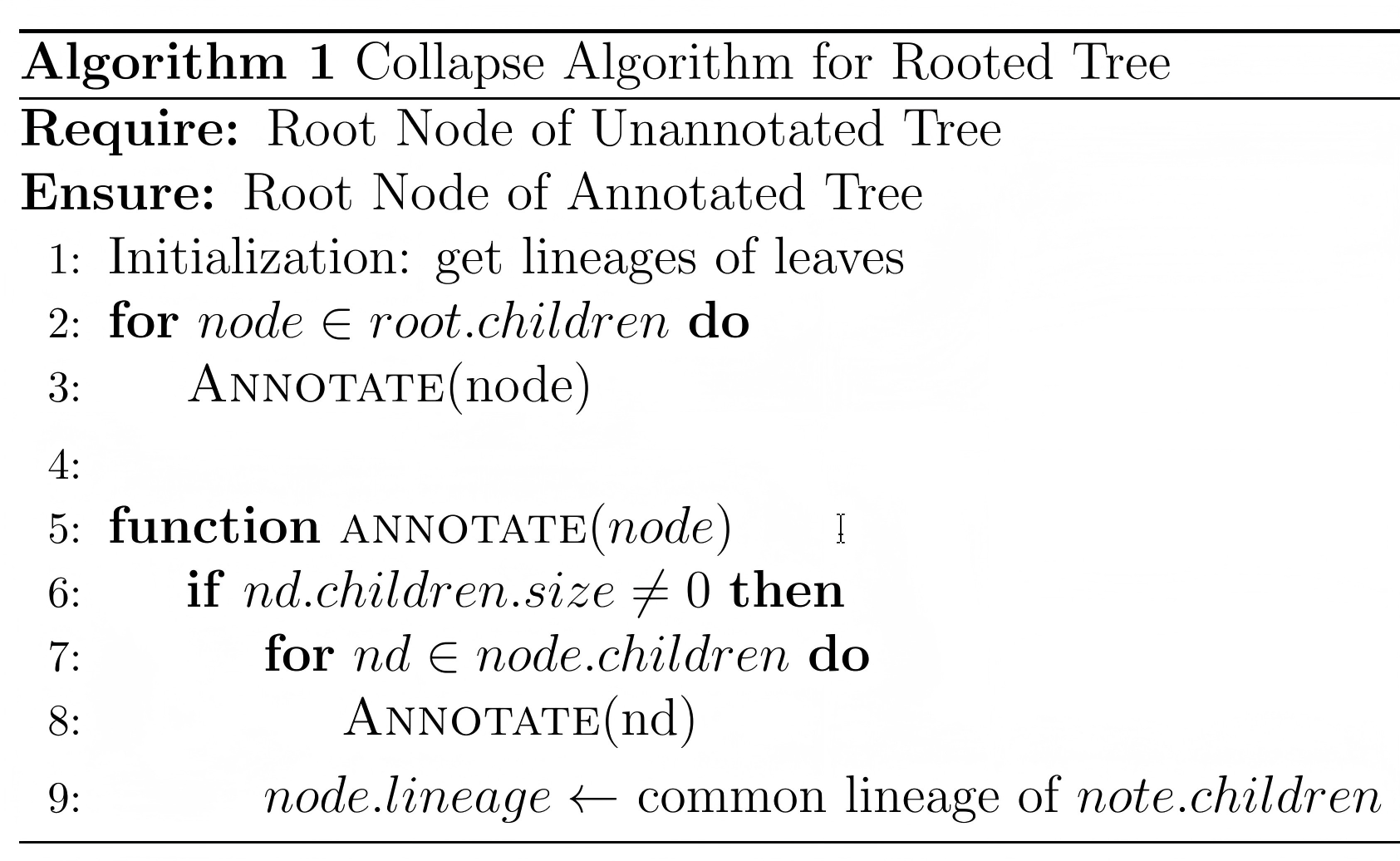
4.2.2 Annotating Rooted Phylogenetic Tree

After obtain the lineage of all leaves of the phylogenetic tree, a rooted tree can be annotated by a recursive algorithm, which named as “Collapse” algorithm. The pseudo-code was show below:

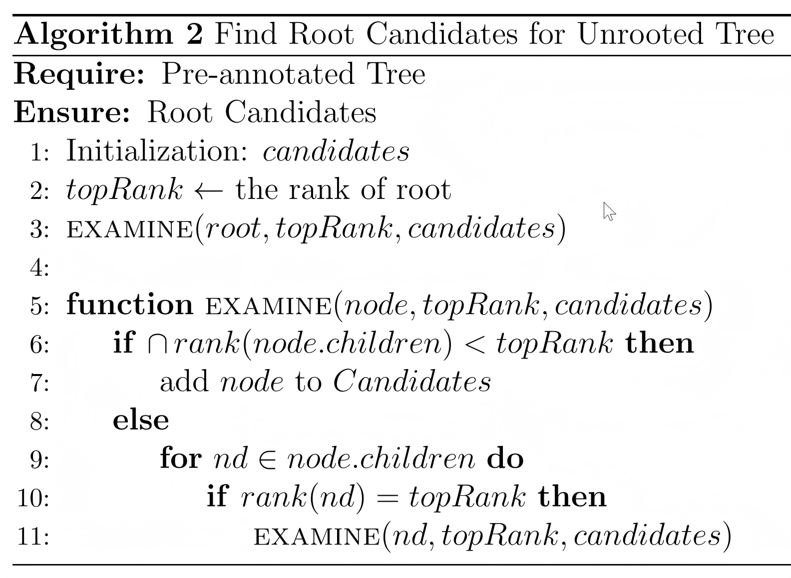
4.2.3 Rooting the Unrooted Phylogenetic Tree

The collapse algorithm can only annotate the rooted tree, due to the taxonomy of biology is a hierarchic classified system. In the CLTree system, there are three methods to annotate a unrooted phylogenetic tree:

• Rooting the phylogenetic tree to obtain the best consistency between the phylogenetic tree and taxonomy, and rearrange the tree to keep the operational taxonomic units (OTU). This is the default method of CLTree.
• Rooting the tree by branch length, five rooting methods are provided by CLTree, i.e. minimal variance (mv, default), minimal ancestor deviation (mad), midpoint (mp), pairwise midpoint root (pmr), minimal depth (md). For more about the phylogenetic method, please refer the reference (Farris, 1972; Mai, Sayyari, & Mirarab, 2017; Tria, Landan, & Dagan, 2017)
• Set a leaf as the out-group for the phylogenetic tree manually (Kluge & Farris, 1969).

The last two methods had been described by other references. The first method, which is firstly provided by CLTree, is a method based on both lineage and branch length of the tree. In this method, a root with the best consistent with the lineage. Here the degree of consistency is measured by the entropy reduction ratio in the CLTree system (see the next section). And basic idea of the method is that:

1. Random select a leaf as the out-group, and annotate the tree by Algorithm.
2. Obtain the root candidates by Algorithm . And select a candidates as the root, rearrange the tree.
3. Annotate the new subtree.
4. Set taxon level as operational taxonomic units (OTU), and determined the final root by a phylogenetic rooting method, e.g. minimal variance (mv, default), minimal ancestor deviation (mad), midpoint (mp), pairwise midpoint root (pmr), minimal depth (md).

5 Development History

The CV approach was first announced in 2002 at C. N. Yang’s 80th Birthday Conference (Hao, Qi, & Wang, 2003) and applied to coronovivuses (Gao et al., 2003) and prokaryotes (J. Qi et al., 2004). Since the publication of the paper (J. Qi et al., 2004), many groups had implemented the classical CVTree algorithms. Here we list the major versions which implemented by our group, and the version numbers of the Standalone CVTree were reset by the version number of the Web Server CVTree as the standalone CVTree have never published:

1. Most 0.x Standalone CVTree was written by Lei Gao; Ver. 0.9.6 was written by Ji Qi.
2. Web Server CVTree v1 was written by Ji Qi, Hong Luo, and Bailin Hao
3. Standalone CVTree 1.x was written by Zhao Xu
4. Web Server CVTree v2 was written by Zhao Xu and Bailin Hao
5. Standalone CVTree 2.x was written by Guanghong Zuo
6. Web Server CVTree v3 was written by Guanghong Zuo and Bailin Hao
7. Standalone CVTree 3.x was written by Guanghong Zuo
8. Standalone CLTree 1.0 was written by Guanghong Zuo
9. Web Server CVTree v4 was written by Guanghong Zuo

6 Acknowledgements

The CVTree project has been supported by National Basic Research Project of China (973 Programs No. 2007CB814800 and No. 2013CB834100), and the Wenzhou institute, University of Chinese Academy of Sciences (Grant No. WIUCASQD2021042).

Reference